Abstract
Context. Precise continuum normalisation of merged échelle spectra is a demanding task necessary for various detailed spectroscopic analyses. Automatic methods have limited effectiveness due to the variety of features present in the spectra of stars. This complexity often leads to necessity of manual normalisation which is time demanding task.
Aims. The aim of this work is to develop fully automated normalisation tool that works with order-merged spectra, and offers flexible manual fine-tuning, if necessary.
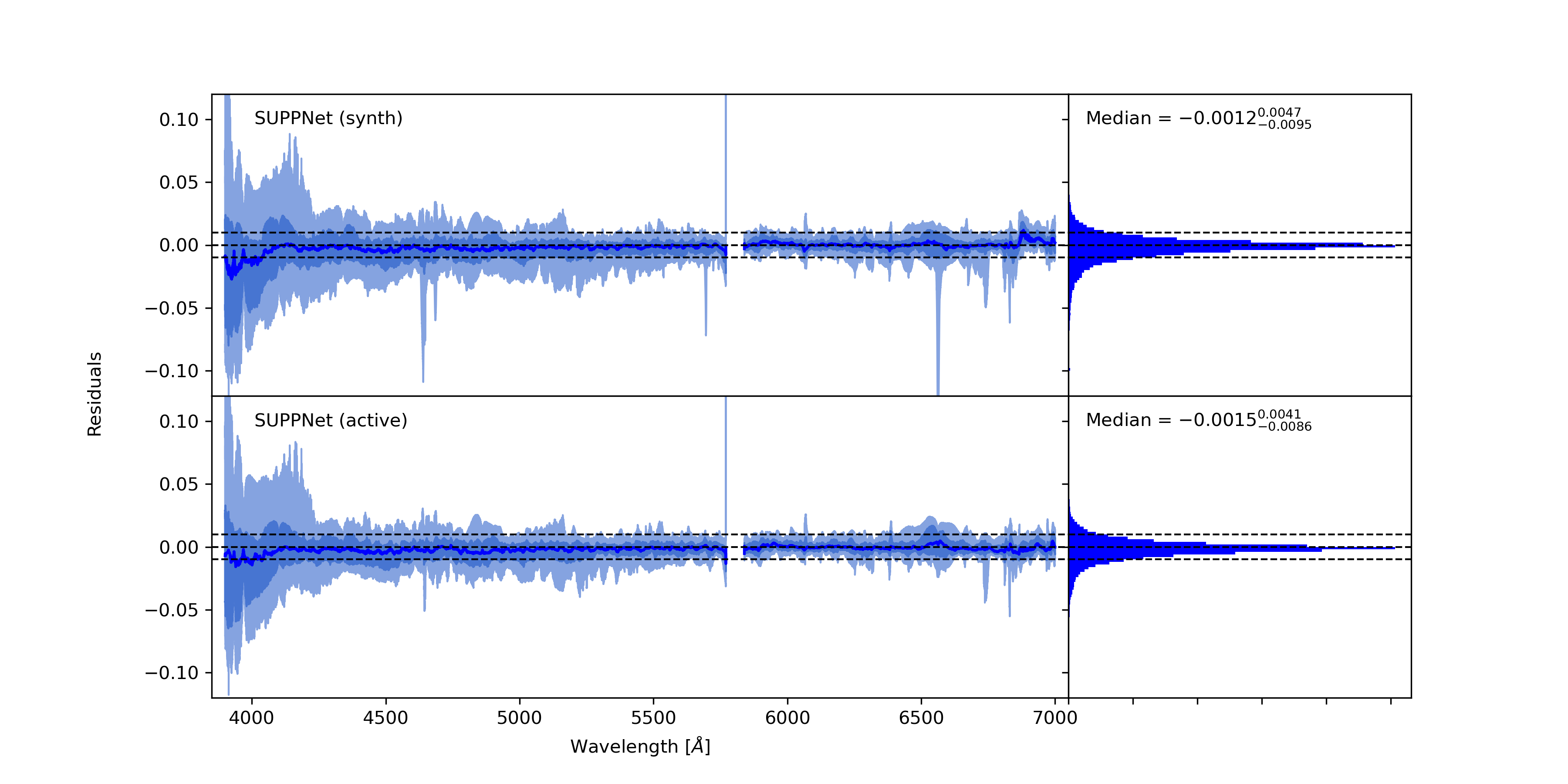
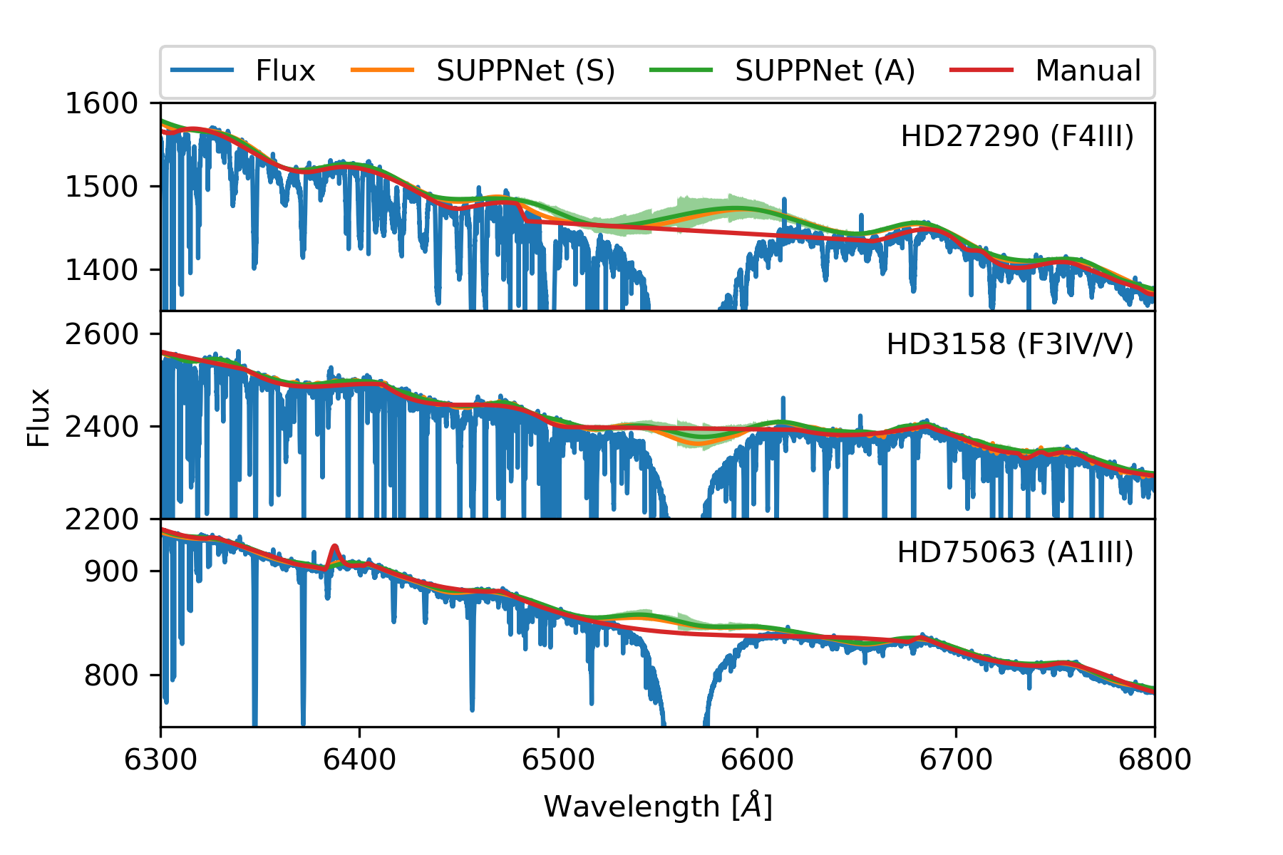
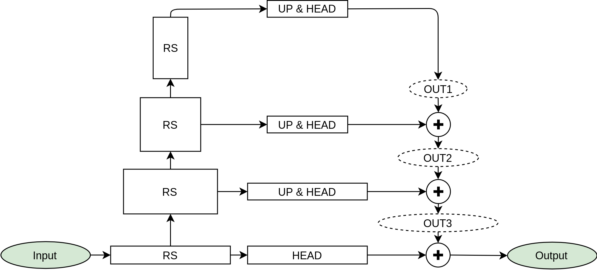
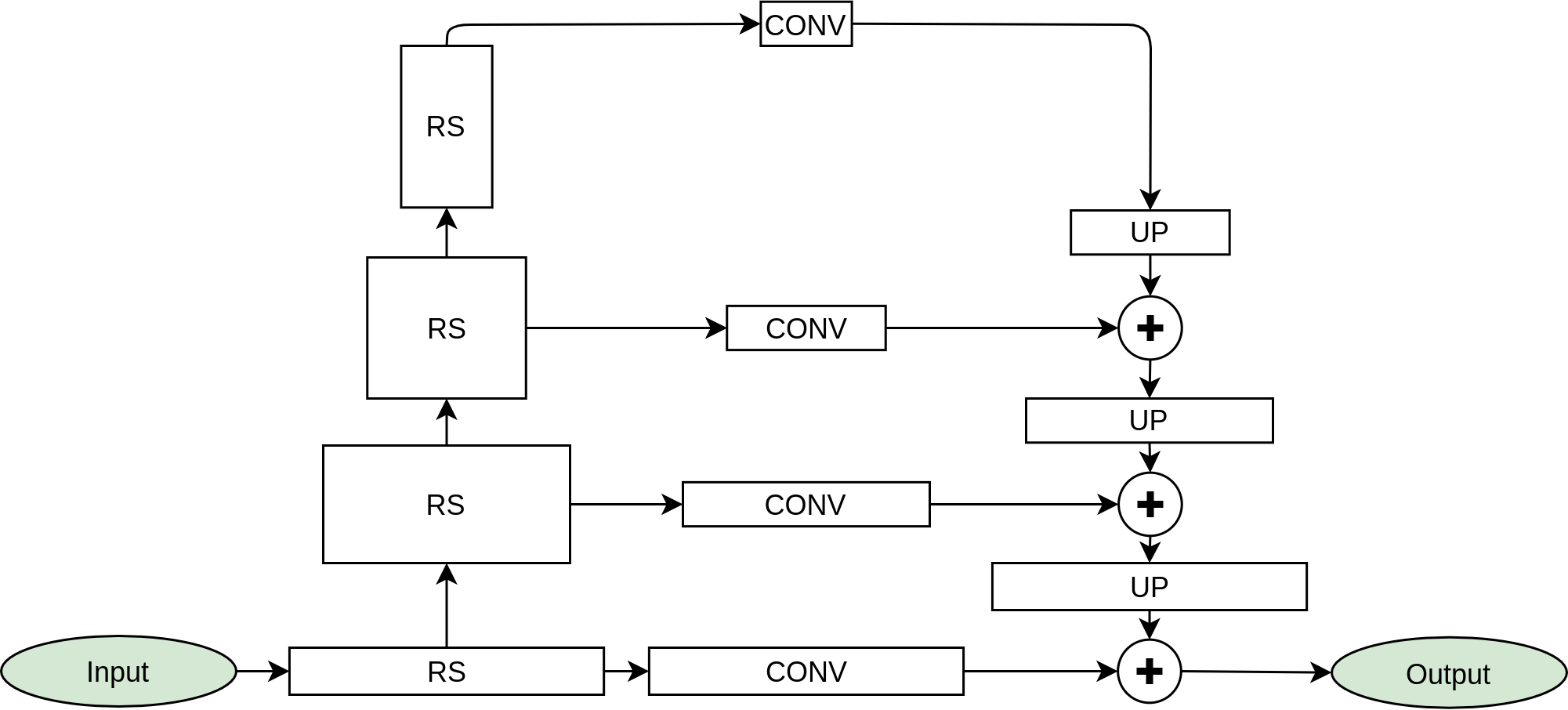
Methods. The core of proposed method uses the novel deep fully convolutional neural network (SUPP Network) that was trained to predict the pseudo-continuum. The post-processing step uses smoothing splines that gives access to regressed knots useful for optional manual corrections. Active learning technique was applied to deal with possible biases that may arise from training with synthetic spectra, and to extend the applicability of the proposed method to features absent in such spectra.
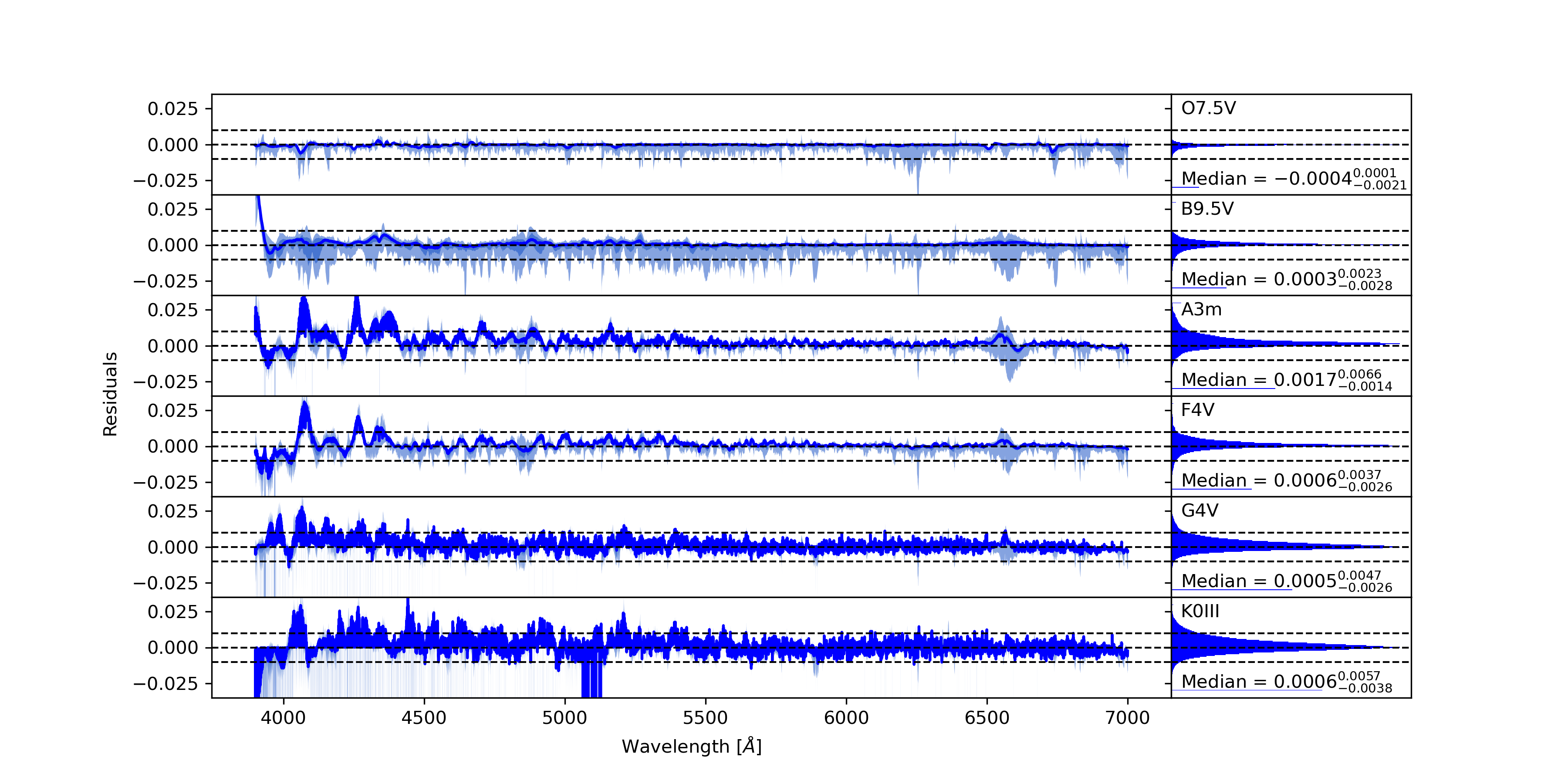
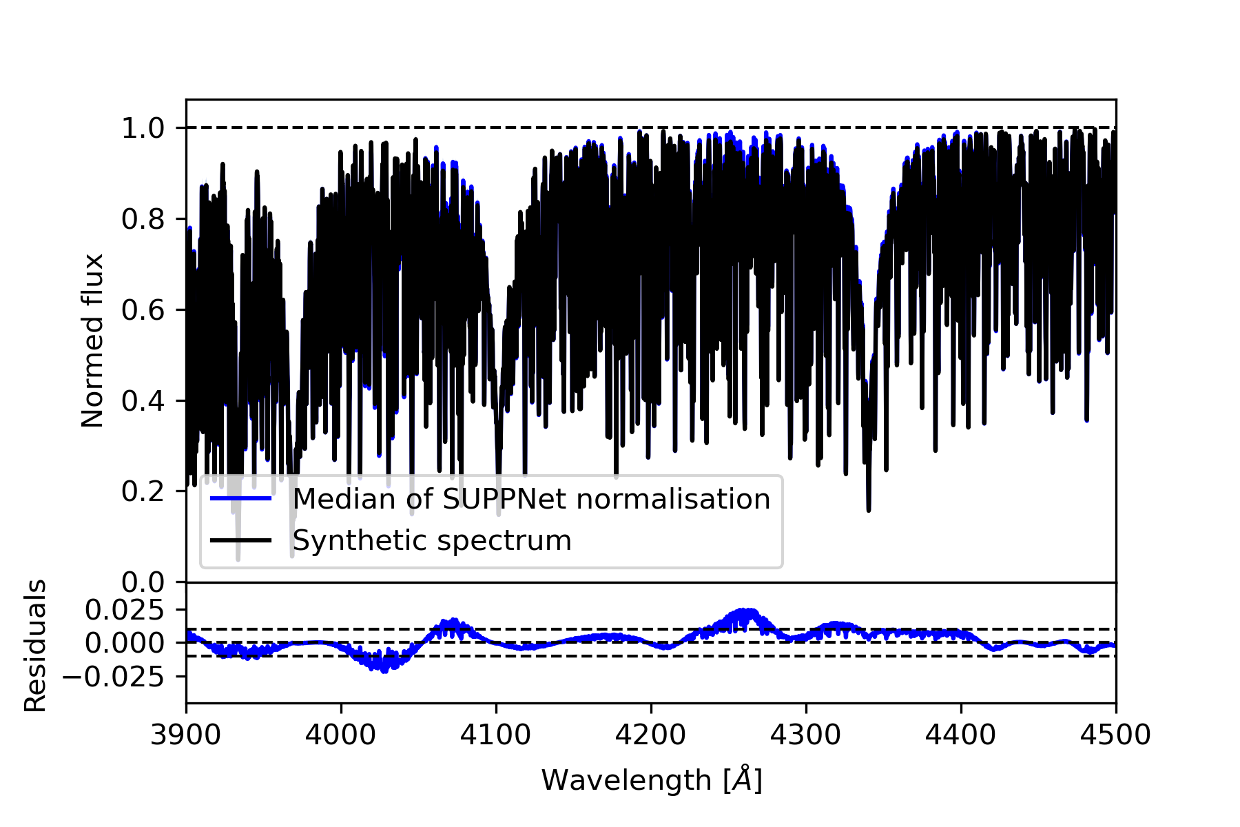
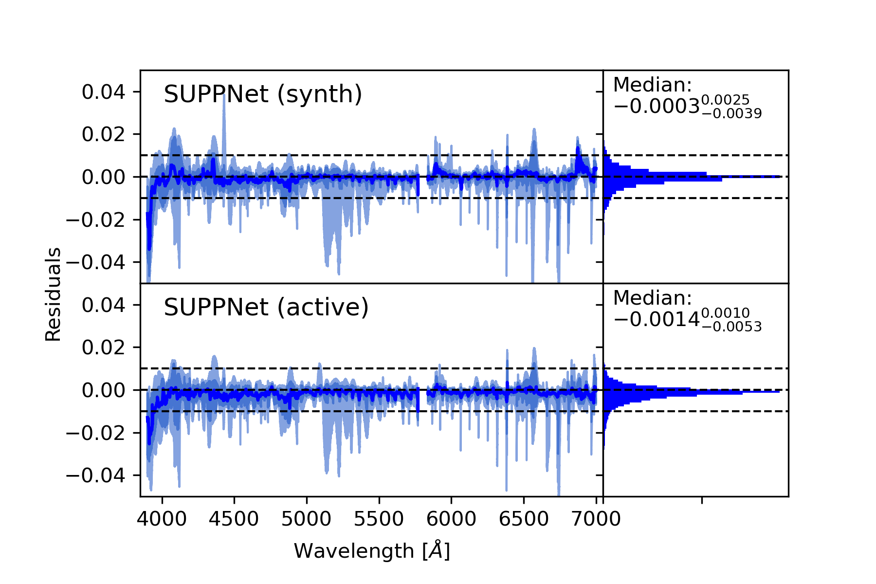
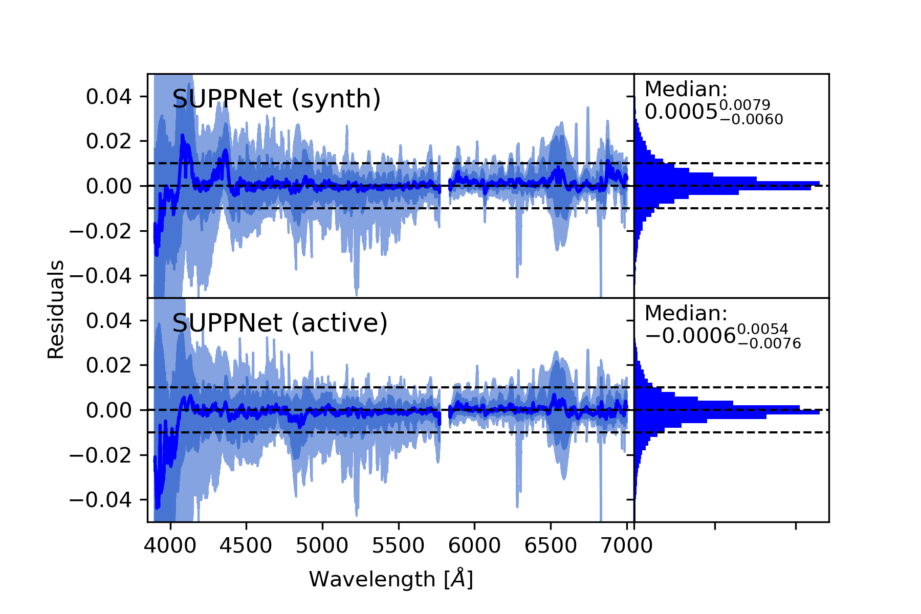
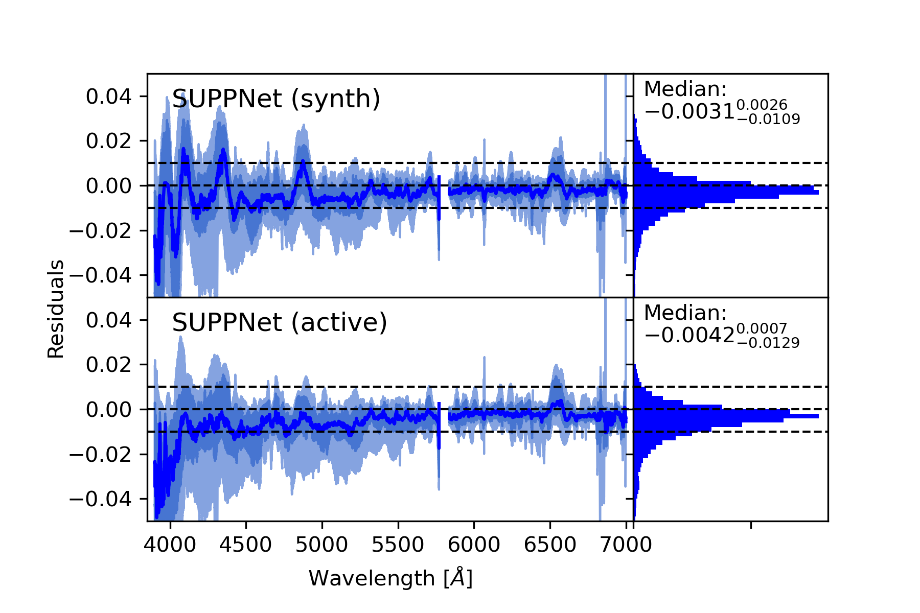
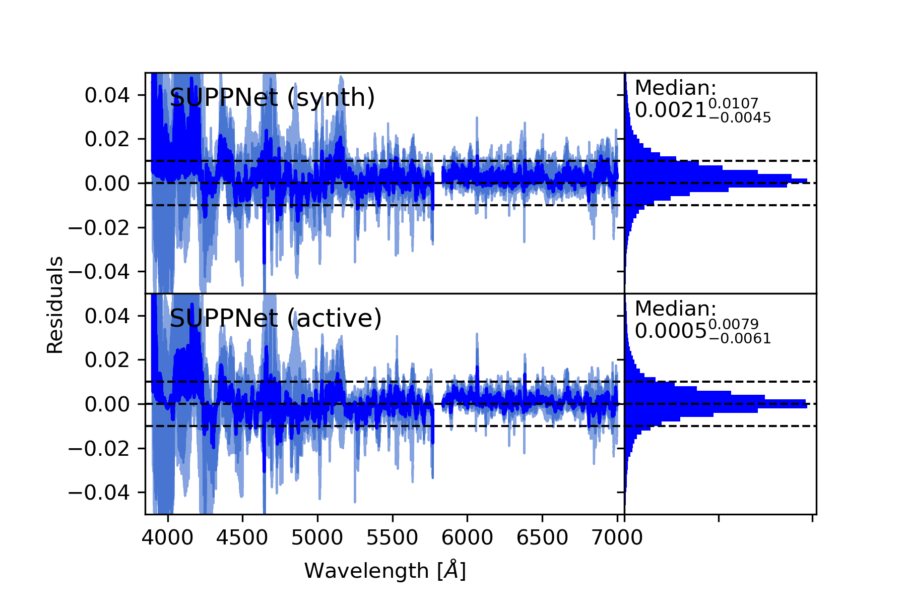
Results. Developed normalisation method was tested with high-resolution spectra of stars with spectral types from O to G, and gives root mean squared (RMS) error over the set of test stars equal 0.0128 in spectral range from 3900 Å to 7000 Å and 0.0081 from 4200 Å to 7000 Å. Experiments with synthetic spectra give RMS of the order 0.0050.
Conclusions. The proposed method gives results comparable to careful manual normalisation. Additionally, this approach is general and can be used in other fields of astronomy where background modelling or trend removal is a part of data processing. The algorithm is available on-line: https://git.io/JqJhf.